Stop Using Zip Codes for Geospatial Analysis

Originally published on CARTO and Towards Data Science in August 2019

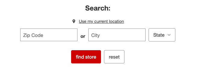
The last time you used your zip code, you were most likely entering your address into a website to make a purchase, finding a store near your home or office, or filling out some other online form. You likely found the answer you were looking for and didn’t stop to think further about that five-digit code you’d just typed out.

However, lots of companies, marketers and data analysts spend hours looking at zip codes. They are deciding how to use data tied to those zip codes to understand trends, run their businesses, and find new ways to reach you, using that same five-digit code.

Even though there are different place associations that probably mean more to you as an individual, such as a neighborhood, street, or the block you live on, the zip code is, in many organizations, the geographic unit of choice. It is used to make major decisions for marketing, opening or closing stores, providing services, and making decisions that can have a massive financial impact.

The problem is that zip codes are not a good representation of real human behavior, and when used in data analysis, often mask real, underlying insights, and may ultimately lead to bad outcomes. To understand why this is, we first need to understand a little more about the zip code itself.

The Zip Code: A brief history

The predecessor to the zip code was the postal zone, which represented a post office department for a specific city. For example:

Mr. John Doe

515 Hennepin Avenue

Minneapolis 16, Minnesota

“16” represents the postal zone in Minneapolis. But with more and more mail being sent, in 1963 the Postal Service decided to roll out the Zone Improvement Plan, which transformed addresses to look like the following:

Mr. John Doe

515 Hennepin Avenue

Minneapolis, MN 55416

The five-digit code represents a part of the country (5_ _ _ _ ), a sectional center facility ( _ 5 4 _ _ ), and the associate post office or delivery area (_ _ _ 1 6).

By 1967 ZIP codes were made mandatory for bulk mailers and continued to be adopted by almost anyone sending mail in the US. Over time, the ZIP+4 was added to add more granularity to the zip code to denote specific locations, even buildings for postal workers to deliver. The Postal Service even created a character, Mr. Zip, to promote the use of ZIP codes, who was featured on stamps, commercials, and songs.

ZIP codes themselves do not actually represent an area, rather a collection of routes:

Despite the geographic derivation of most ZIP Codes, the codes themselves do not represent geographic regions; in general, they correspond to address groups or delivery routes. As a consequence, ZIP Code “areas” can overlap, be subsets of each other, or be artificial constructs with no geographic area (such as 095 for mail to the Navy, which is not geographically fixed). In similar fashion, in areas without regular postal routes (rural route areas) or no mail delivery (undeveloped areas), ZIP Codes are not assigned or are based on sparse delivery routes, and hence the boundary between ZIP Code areas is undefined.

The US Census provides data for ZIP Code Tabulation Areas, or geographic files:

ZIP Code Tabulation Areas (ZCTAs) are generalized areal representations of United States Postal Service (USPS) ZIP Code service areas.

The USPS ZIP Codes identify the individual post office or metropolitan area delivery station associated with mailing addresses. USPS ZIP Codes are not areal features but a collection of mail delivery routes.

Sign up for my once a month newsletter

[mailerlite_form form_id=2]

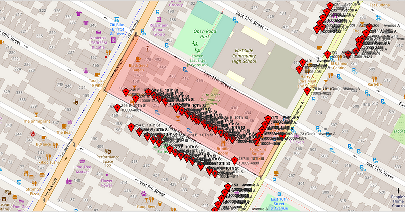
Here we find our first problem with ZIP Codes, that they do not represent an actual area on a map, but rather a collection of routes that help postal workers effectively deliver mail. They aren’t designed to measure sociodemographic trends, as a business would generally want to do. You can actually look up individual delivery routes, like the one below:

We are only scratching the surface of the issue here. Similar issues exist around the world, with postal codes representing strange boundaries:

Using ZIP codes for data analysis

Fast forward to today, where many companies can easily look into their database and find a dataset with a zip_code column in it, which allows them to group and aggregate data to see trends and business performance metrics. As stated earlier, the problem with ZIP Codes is that:

1. They don’t represent real boundaries, but rather routes
2. They don’t represent how humans behave

The latter represents two specific issues in using spatial data: spatial scale of observations and spatial scale support (you can learn more about this in this lecture from UChicago’s Luc Anselin, here). The first is that humans don’t behave based on administrative units such as zip codes, or even census units. Their behavior is influenced much more by their neighbors, or areas such as neighborhoods or high activity areas (such as central business districts). The second is that spatial data is provided at multiple scales, and many times those boundaries are overlapping or nested within another boundary.

Let’s look at an example of this in one specific area in Dallas.

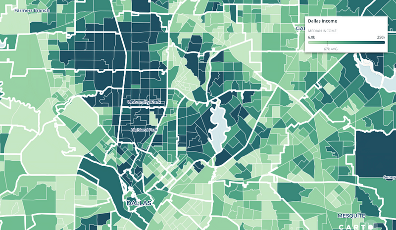
In this map, we can see large white boundaries, which represent ZIP code boundaries, and below them are boundaries for US Census Block Groups. The darker green represents higher income, as provided by the US Census.

When we look at one specific ZIP Code we can see that income data in even more detail:

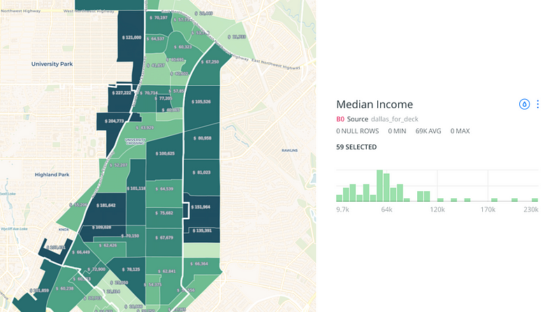
What we can see is that 12-month median household income in this single zip code (75206) ranges from $9,700 to $227,000 when we look at block groups that completely or partially fall within this single ZIP Code, which the Census lists as having a median household income of $63,392.

Median Income is one way to evaluate the range of values within a ZIP Code (keep in mind these are ZCTA boundaries) but we can likely see variance like this in population, employment, and other relevant metrics for data analysis.

Sticking with median household income, we decided to expand this analysis to the entire United States, to see which areas are the least and most in-equal when you look at ZIP Codes and the Census Block Groups that intersect with the ZCTA Boundaries that had at least 1 person living in that Block Group.

The most unequal zip code is 33139 in Miami Beach, FL

1. 33139: Miami, FL ($241,344 Difference)
2. 44120: Cleveland, OH ($237,501 Difference)
3. 10013: New York, NY ($233,559 Difference)
4. 10023: New York, NY ($233,157 Difference)
5. 11201: Brooklyn, NY ($233,031 Difference)
6. 10601: White Plains, NY ($232,813 Difference)
7. 33141: Miami, FL ($232,633 Difference)
8. 92648: Huntington Beach, CA ($231,290 Difference)
9. 98105: Seattle, WA ($230,906 Difference)
10. 33143: Miami, FL ($230,626 Difference)

The most similar* zip code is in Chesapeake, WV

1. 25315: Chesapeake, WV ($2 Difference)
2. 79357: Cone, TX ($4 Difference)
3. 65052: Linn Creek, MO ($9 Difference)
4. 73093: Washington, OK ($12 Difference)
5. 68370: Hebron, NE ($13 Difference)
6. 19541: Mohrsville, PA ($15 Difference)
7. 05340: Bondville, VT ($18 Difference)
8. 12958: Mooers, NY ($26 Difference)
9. 19941: Ellendale, DE ($37 Difference)
10. 54896: Loretta, WI ($38 Difference)

*similar where the difference is greater than 0

To perform this analysis for the entire United States, I used CARTO and its notebook extension CARTOframes to pull in census data for Census Block Groups and Census ZCTA areas, which are stored in CARTO.

Once we had both sets of boundaries, we want to look at all block groups that are either completely contained by a ZCTA boundary, or at least 50% contained by a ZCTA boundary. To do that we can use PostGIS to find those intersections as well as create different statistical measures from that data (min, max, and percentiles).

You can see the complete methodology and code in this notebook.

SELECT
z.*,
MIN(b.median_income),
MAX(b.median_income),
SUM(b.total_population) AS total_pop,
percentile_disc(0.25) WITHIN GROUP (ORDER BY b.median_income) AS p_25,
percentile_disc(0.5) WITHIN GROUP (ORDER BYb.median_income) AS mean,
percentile_disc(0.75) WITHIN GROUP (ORDER BYb.median_income) AS p_75,
stddev_pop(b.median_income)
FROM
income_zips z
LEFT JOIN income_bgs b 
ON ST_Intersects(z.the_geom, b.the_geom)
WHERE
b.total_population > 0
AND (ST_Area(ST_Intersection(z.the_geom, b.the_geom))/ ST_Area(b.the_geom)) >.5
GROUP BY
z.cartodb_id

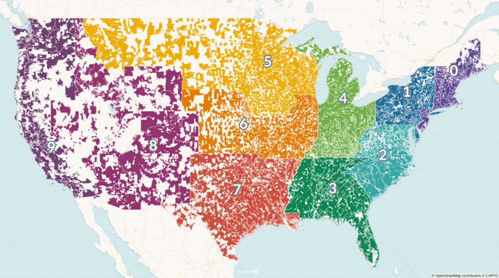
After creating this as a new table we can see that the majority of the most unequal zip codes tend to be in cities or larger metro areas and more equal zip codes tend to be in rural areas around the country.https://forrest.nyc/media/f0b8ac02c7b9381c125236425dcbcc2b

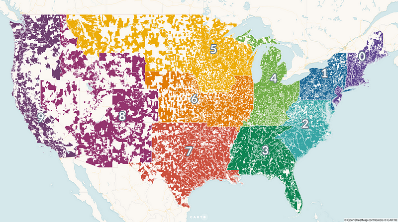
It’s also worth exploring spatially significant clusters of zip codes based on their range between the highest and lowest values, which is a perfect fit for using spatial autocorrelation. You can learn more about it in this article or in this tutorial.https://forrest.nyc/media/e25b2e973633e996ecc659bb3b038404

So why do we use ZIP Codes?

In practice, it is easy to use zip codes as a geospatial unit. As we stated earlier, almost any e-commerce or delivery service, or app that uses location or needs to locate their users in any way will collect a zip code. Additionally, everyone is familiar with zip codes, as they are part of any address in most countries.

Terms like Census Block Group or Tract are less familiar to those who don’t work with geospatial data on a regular basis, and they can be more difficult to find and harder to work with, especially if you aren’t familiar with terms like Shapefile, FTP, and ETL. Even then you have to go through the US Census FTP website, download geographic files state by state, and join those files to census measures.

Finally, most people know, without looking at a map that zip codes represent a smaller area than a city, but larger than say a neighborhood. Conceptually, they feel small enough to get a very focused view of the world, and big enough to capture enough of a sample size of trends.

The short answer is that zip codes are easy to find, familiar, and provide a granular enough view of the world (or so we thought).

With that said there are real-world problems that arise from using zip codes in geospatial analysis. One example is in real estate where, in many cities or areas, there are homes listed in a ‘desired’ zip code, even though as we know those boundaries are arbitrary. This article from the Harvard Business Review also describes a similar phenomenon with Airbnb listings and rising rent prices.

In simple terms, we argue that if a zip code is “touristy,” meaning it has a lot of restaurants and bars, and if awareness of Airbnb increases, which we measure using the Google search index for the keyword “Airbnb,” then any jump in Airbnb supply in that zip code is likely driven by an increase in demand for short-term rentals through Airbnb, rather than local economic conditions.

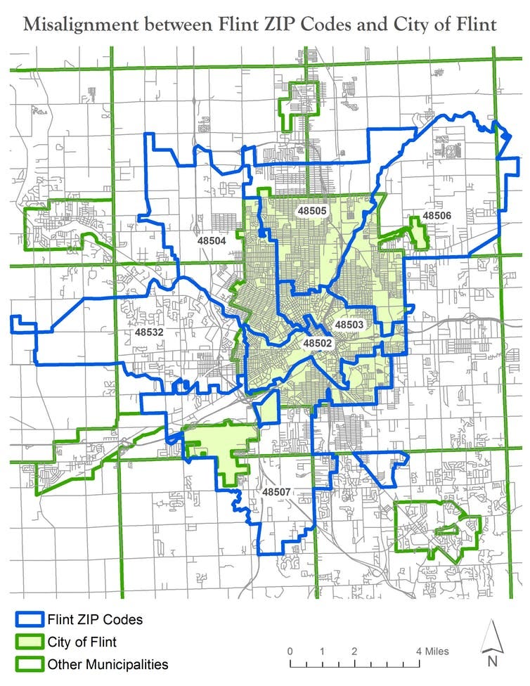
More importantly, using zip codes for analysis can mask serious conditions that are taking place at a different spatial scale. The Flint water crisis was one of these cases. This article by Richard Casey Sadler, an Assistant Professor at Michigan State University describes the problem in great detail and raises similar points about zip codes (the full article is well worth reading):

Dr. Tony Grubesic, an Arizona State University professor, has called them “one of the quirkier ‘geographies’ in the world.” Dr. Nancy Krieger, a Harvard University professor, and colleagues have called out their unacceptability for small-area analyses.

Ultimately the state used zip codes to analyze the blood lead statistics in aggregate, which effectively masked the actual issue. This is because:

In Flint’s case, the state’s error was introduced because “Flint ZIP codes” do not align well with the city of Flint or its water system. The city and water system are almost 100 percent coterminous — that is, they share the same boundaries… In total, Flint ZIP codes used in the state’s analysis blanket parts of eight different municipalities (seven townships and one city) surrounding Flint.

In the case of Flint, simply looking at a different spatial scale or analysis may have shown the problem more clearly. For fields like public health and critical services, understanding and using appropriate spatial scale is critically important.

What else can we do?

So if you are compelled to do away with zip code analysis, the good news is that there are several different options available.

Use Addresses

The first and foremost recommendation would be to use real-world addresses. When you know an address string, you can use a geocoder — or the service that Google or other map search engines use to take an address and transform it into latitude and longitude. Most every major service offers an API and wrappers for different languages to do this. Keep in mind there are generally some best practices for cleaning your data, and you will need valid address strings to do so. Other tools like Libpostal can help you normalize and parse your address strings.

Use Census Units

You can also use Census units such as a Census Block Group or Tract. As I mentioned it has not always been easy to find and collect this data at scale, but there are many new tools that are becoming available to use. CenPy is a Python library that allows you to connect and find Census data (good tutorial here) where you can find measures from the decennial census or American Community Survey. CARTO also provides Census and ACS through the Data Observatory, which was used in the notebook for the full US analysis.

You can also find out Census geometry IDs for a specific address location using the US Census Geocoder. You can pass in a variety of parameter so the API or use it in Python with the censusgeocode package.

As your gather address data, you can easily add in a Census Tract or Block Group ID to that entry, and use that rather than the zip code field in your data. This will allow you to do the same aggregation you were doing, except at a more appropriate geographic scale.

Use your own Spatial Index

Finally, there are more and more geographic spatial indexing tools than ever. Google uses S2 cells, you can use quadkey indexing for grid cells, and Uber uses H3 hexbins. What is nice about all these libraries is that the children of a parent cell are more evenly contained by the parent to avoid spatial overlap issues. As long as you have a latitude and longitude (which would require geocoding), you can use one of the variety of libraries to assign an ID to that record.

There are two main advantages to using a spatial index. First, you are not locked into any specific boundary type, you can use the same unit of study anywhere on the globe. This allows you to compare trends in a cell in Midtown Manhattan to one in Lagos, Nigeria, as long as the underlying data is the same.

The second is the anonymization of sensitive data. Given that address data can be sensitive, you can create a data pipeline that simply reads incoming addresses, geocodes them, assigns a spatial index, then passes that indexed data into a separate table, then you can store or delete the address data as needed.

Working with spatial data can be difficult, but the availability of data and tools has made it more accessible. By using the correct spatial scale and discarding analysis at the zip code level, you can improve the quality of your insights and create more meaningful outcomes and analysis.

Matt Forrest works at CARTO and has been working in spatial data science for the past 9 years.