Tapping into the power of spatial SQL aggregations

Use aggregations in SQL to group your data and perform large scale spatial joins

Picking up where we left off from our last tutorial, we will jump right into the next set of topics:

• Using the WHERE clause to do more advanced filtering of your data
• Aggregations by grouping your data, filtering aggregated data using HAVING, and using selective aggregations to aggregate only specific sets of data
• Spatial aggregations — or spatial relationships using intersections, contains, overlaps, and unions

But first, a review of our challenge from Part 1

Here is the challenge from the last post:

Using the Mapzen Who’s on First dataset in BigQuery, let’s look for airports located in Canada, and order them by their airport name and their south to north location.

And here is the query:

The first thing we need to do is to filter to results in Canada, so we use the WHERE clause to get all airports that fall in the country of Canada, or ‘CA’.

Next, we need to order by two parameters. The first is airport location by south to north, which we can extract from the geom column using ST_Y, and order it in ascending order using ASC. Finally, we take the airport name, order it alphabetically using ASC.

Now, you could also use the numeric value for the latitude as well, which would likely be more efficient. This is because we are using the data, and not calculating anything in the function ST_Y. Many times in spatial SQL, there may be a more efficient way to calculate a result by storing values as non-geography data types.

In short, if you don’t need to use extra functions, don’t!

Advanced WHERE: Using BETWEEN, IN, and EXISTS

As a follow-up from the last post, there are a few more advanced methods to using the WHERE clause. We can also add other conditions using different keywords such as BETWEEN:

The above query will return all rows from the table where the state name falls between Alaska and Kentucky. BETWEEN works for numbers, strings, and dates.

You can also filter by a set of conditions using the IN keyword:

The above query will return rows where the state_name is either Minnesota, Wisconsin, Iowa, or Illinois. IN and BETWEEN are the two advanced WHERE operators I have used most in my geospatial work, but you can also use EXISTS, ANY, and ALL to query against data in another table should you need.

Sign up to get monthly email updates on all things geospatial

[mailerlite_form form_id=2]

You can use different functions to aggregate data while using GROUP BY

Now, this is where things start to get really fun, especially with geospatial data. GROUP BY allows you to use different functions to aggregate data and then group them by other columns in your data.

First let’s use some more interesting data from the US Census: US Counties with different population data.

Let’s take a look at a few aggregation functions and run them for the entire table: well use AVG, MIN, COUNT, SUM, and MAX:

This will return the respective values for all records in our table. But let’s say we want to group them by another measure in our table, such as state name (we can use state FIPS code for our purposes). We can do this using GROUP BY:

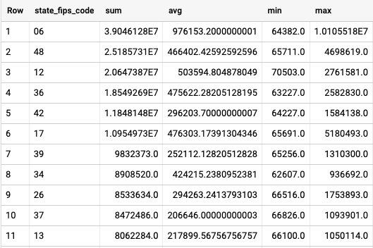
As you can see in the results, we are now grouping the aggregations by the state FIPS code, and we can see the largest state has the code ‘06’ which of course corresponds to California.

There are lots of different aggregate functions, which you can check out here:

We can also perform what is known as a dissolve in GIS using ST_UNION_AGG:

Aggregations is an area where BigQuery and other data warehouses perform well, especially with large-scale data.

Filter aggregated columns using HAVING and selectively filter aggregated data

In aggregations, you can’t use the WHERE clause to filter your aggregated values, such as items where the COUNT is greater than a specified number. To do that we can use HAVING:

You can also do this in the aggregation function using the CASE syntax. CASE allows you to write statements such as “if value x, then return 1, if value y, then return 2…else return 0.

You can do this inside an aggregate function such as SUM or AVG. PostgreSQL provides a simpler syntax called FILTER to do this and if you are using BigQuery, you can use COUNTIF for count aggregations.

In this case, we can get the average total population of counties in each state, for just counties that have populations over 500,000.

Aggregations with spatial data fall into a few common use cases

There are plenty of times you might use aggregations with spatial data, but in my experience, I would group the majority into five main use cases:

1. Aggregating data across a single table that contains unique geography data – either non spatial data and/or using ST_UnionAgg to aggregate geometries
2. Aggregating data across a single table with multiple entries with the same geometry – often times a time series dataset with geometries that repeat
3. Aggregating longer, non-spatial data to a spatial dataset
4. Spatial join between two tables with geospatial data using spatial relationships
5. Using spatial relationships to evaluate aggregated data from another table for each row of the source table

Each of these use cases uses some concepts that we haven’t covered yet, but this will help you understand how to use aggregations in a spatial context.

Aggregating data across a single table that contains unique geography data

For the first use case, we can use our US counties example to aggregate data by state name.

To make this more interesting let’s remove all counties with a pop density of less than 500 per square mile, and union the geometries together, grouping by the state name.

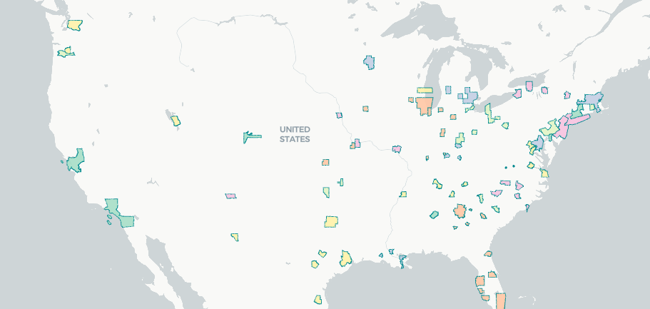
This data only has one unique geometry per row, which differs from our next use case.

Aggregating data across a single table with multiple entries with the same geometry

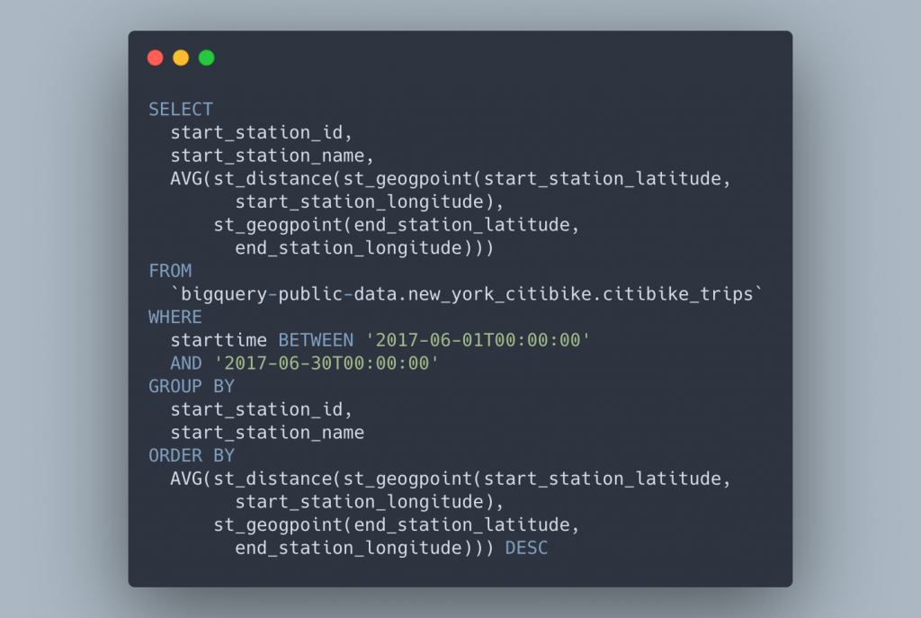
Next, let’s take a look at CitiBike trips in New York. In this dataset, there are many trips but a discrete set of stations, and a discrete set of geometries to match.

For this use case let’s calculate the average straight-line distance traveled between the start and end stations for all stations.

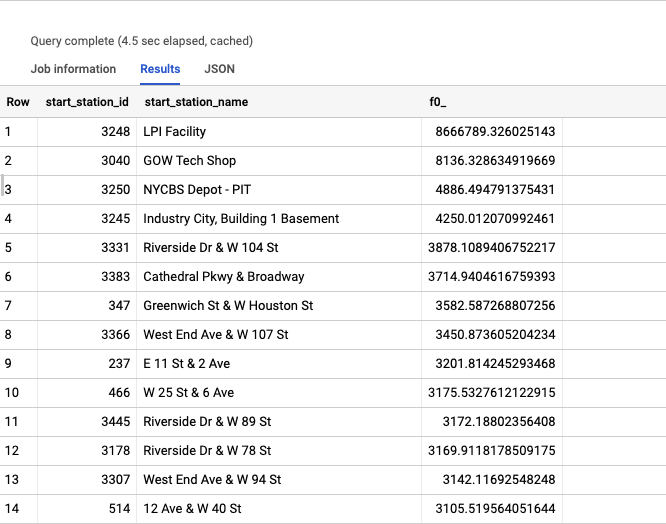
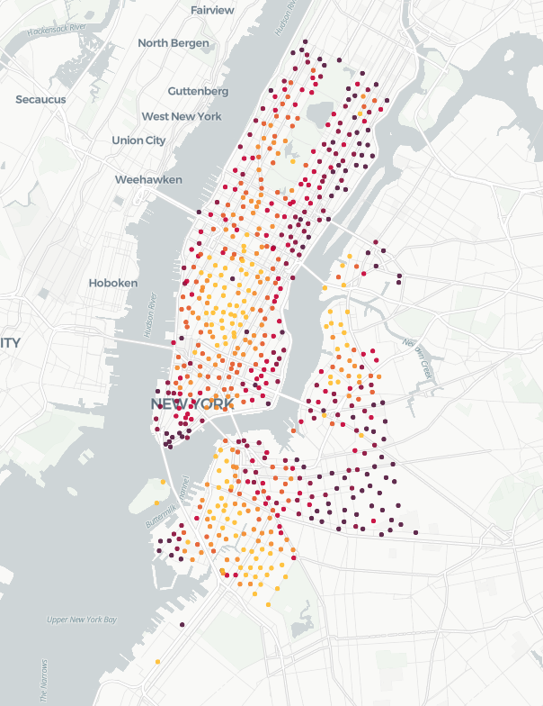
As you can see, we can aggregate across the entire dataset, but group by a single common geometry. Even though the geometry (albeit in this case a set of lat/longs), we can group by that single common record.

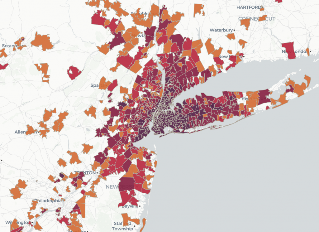
Aggregating longer, non-spatial data to a spatial dataset

In the next use case, imagine we have a long dataset of repeating records with an ID that can be tied to a single geometry. This could be time-series data or maybe sales by postal code by week.

We can use New York City’s 311 data to demonstrate this. Each record includes a ZIP code where the call was reported. We can join this to a dataset containing ZCTA geometries

Spatial join between two tables with geospatial data using spatial relationships

This will be the most familiar query for someone coming from a pure geospatial background. This query will perform a spatial join, meaning we have two tables both with a geometry value. Usually one of these tables contains a polygon.

For this case, we can aggregate taxi trips in New York by H3 cells.

In a future post, we will explore spatial joins in more detail and how you can perform them in different tools and languages.

Using spatial relationships to evaluate aggregated data from another table for each row of the source table

The final use case is, row by row, exploring some aggregated data of values using a spatial relationship. One example here is looking at the median income of areas that touch a target area, or neighbor analysis. We can do this using a subquery, specifically a correlated subquery.

If you are using PostgreSQL/PostGIS, you can use the LATERAL keyword. There is a great post from Paul Ramsey that explains this in detail for nearest neighbor bulk joins.

Spatial SQL Challenge: Perform an aggregated spatial relationship analysis with different aggregations

There will be two challenges for this section:

First, using roads and US Counties, find the count of interstates, and the interstate names for each state that solely fall within one state. A quick hint: there is a specific spatial function that looks for geometries that are entirely contained by another.

Second, using the New York Taxi Trips dataset and US Census Block Groups we are going to find the:

• Total number of taxi trips in each census block group in New York that has
• Tips higher than 20% of the total
• Where there are at least 50 trips started
• Between June 1 and June 7, 2015