Join all the things in spatial SQL - Matt Forrest - Modern GIS and Geospatial Ideas and Guides

In this post, we will take a look at joining data in SQL. We will take a quick look at joining data in SQL generally, and then how to perform spatial joins using spatial relationships.

Let’s take a look at the answers to the challenges from the previous post

If you are following along, in our previous post we had two challenges using aggregated data.

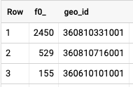
First, using US roads and US States, find the count of interstates, and the interstate names for each state that solely fall within one state.

The function we need to use in this case is ST_Contains, which is defined as:

ST_CONTAINS(geography_1, geography_2)

Returns TRUE if no point of geography_2 is outside geography_1, and the interiors intersect; returns FALSE otherwise.

So, using the roads dataset, we can search for roads that begin with ‘I-‘ which is how the roads are named in the table (you will have to search for that a bit). And since we don’t want to include things like ramps and other smaller roads, let’s limit our roads to anything over 5km.

But, as we can see from the results, there are lots of interstates that fall within one state and multiple repeat values. Why?

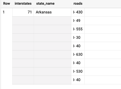
The roads are stored in segments and also clipped to state borders. So there is an I-5 in California, Washington, and Oregon.

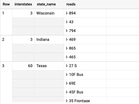
We can use ST_Union_Agg to group our geometries by road name, and then intersect it with the state boundaries, giving us the following results:

For our second challenge, we want to analyze NYC Taxi Trips by US Census Block Group where:

Total number of taxi trips in each census block group in New York that has
Tips higher than 20% of the total
Where there are at least 50 trips started
Between June 1 and June 7, 2015

So, let’s take a look at the query and break it down, step by step.

This was a complicated challenge, so kudos for giving it a try!

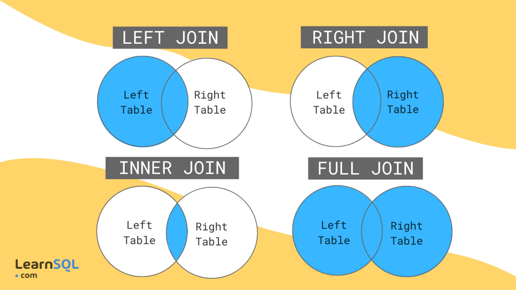
There are many different types of joins in SQL

A join us just what it sounds like, taking records from two or more tables, and joining them together using common column(s) in each dataset.

Here is a very brief overview of the different SQL join types.

Inner Join

An inner, or natural join, returns rows that match the join condition from both tables.

It’s one of the more common joins and can be called using INNER JOIN, or simply, JOIN.

Left Join

The next three types of joins are known as outer joins since they return all the rows from one table, and some from the other table. Where no matches exist, NULL values are returned.

The left join returns all the rows from the left table, even if no values from the right table match.

Right Join

And the exact opposite of a left join is of course a right join, where all rows are returned from the right table, even if no values from the left table match.

Outer Join

An outer join, or full (outer) join, will return the combination of the right and left joins. This means that the results that match between the tables, and the values that do not match from both tables will be returned.

Cross Join

This is a less frequent type of join, but one that has some specific use cases for geospatial data. The cross join returns the Cartesian result of all rows to all other rows, or that all possible combinations of rows would be returned. So if you had two tables of 3 rows, a cross join would return 9 rows.

There are lots of examples and tutorials of joins, so I put together a few of my favorites here.

Spatial joins use all different types of joins

Setting aside use cases such as joining raw or aggregated data from one table to a table with geospatial data (covered in my last post), there are several different ways to use spatial joins – where we create a join based on a spatial relationship.

These spatial joins generally use any of the spatial relationship functions, that evaluate two different geometries (note: the below list represents functions currently contained on BigQuery):

There are some great resources that explain the differences between the different functions such as this post by Michael Entin (who has a lot of great geospatial resources for BigQuery).

One of the most common spatial joins will be a spatial intersection, evaluating which geometries fall within another geometry. To do this we can take a look at US Census Block Group polygons and New York City Taxi Trip data.

Before you start running your queries, I would recommend making a new table using the below query. This will make a copy of the NYC Taxi Data for a short date range, but also create a true GEOGRAPHY column, which is a best practice to help speed up your queries.

Spatial join using a SQL join

Before we write any queries, let’s take a look at what ST_Intersects actually does. Borrowing from the BigQuery docs:

ST_INTERSECTS(geography_1, geography_2)

Returns TRUE if the point set intersection of geography_1 and geography_2 is non-empty. Thus, this function returns TRUE if there is at least one point that appears in both input GEOGRAPHYs.

There are a few ways to use these functions, such as adding intersected polygon values to points (can you name the join type we are using):

The key is that the function will return true or false, which allows us to use it a few different ways. However, the most efficient way is to use a join, like this query below, which uses an aggregation with a join:

Since our ST_Intersects function will return true, we can actually use that as the condition for our join. If you think about other SQL joins, they are evaluating the same thing:

on a.column = b.column

# where this returns true, it joins, false, it does not

Now it is important to consider which type of join you want to use. If you just want the geometries from both tables that intersect, an inner join will be just fine. However, if you want to include the rows from the left table that don’t have a match from the other table, a left join will be the way to go.

Now if you want to join two or more tables to a set of geometries there are some different strategies to put in place. Let’s take a look at a sample query:

Now, let’s join our same dataset, again.

One would think we could just keep using our inner join but…

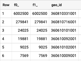
We can see here from the results that our values are way out of proportion compared to our first query. Why is this?

In short, each table join will return a single, intermediate table, also known as a derived table. The multiple joins will read each step sequentially, so in the case above when we reference our second join to the first table, we are inadvertently returning a Cartesian join, or cross join, because one table may match 50 geometries in the first join, while the second could match 1000, for example.

My personal choice for avoiding this is using common table expressions or CTEs. We will cover them in-depth in a future post but for now, you can learn more about them here.

The reason being is that in most cases, we want to compare or join one table that contains our target geometries (in this case our Census Block Groups) to two or more tables containing other geometries. Since we would have to keep reaching back to our first table, and there isn’t a great way of knowing how many intersections each join will produce.

Using CROSS JOINS for spatial relationships

The cross join has some interesting use cases in spatial SQL. The first is building an origin-destination matrix. We will use our NYC taxi trip start points here as an example, to calculate the straight line distance from every station to every station:

You can also use routing functions to accomplish the same task, such as those in the CARTO Spatial Extension, to calculate by driving distance.

The other use case is one that I have used many times. In standard SQL, we can use the cross join to create a row by row join to evaluate spatial relationships from another dataset. A few examples of this are:

Getting min/max/average/count values from polygons touching the target polygon
Find the min/max/average/count of N nearest neighbors
Get the name or value from the nearest neighbor
Get the min/max/average/count of all values within a certain distance

In PostGIS, you can achieve the same thing with a simpler and more efficient process using the LATERAL keyword as outlined here in this blog post by Paul Ramsey.

In this use case, we will take a look at US counties and get the average median income of the counties that touch the target county. Using a cross join, we can limit our results by first selection results that touch the target geometry and that don’t match the target (so we don’t include the target in the calculation).

This is a super useful query and one that I have used time and time again to help study the effects of neighboring areas on a target area, and it is also very helpful for creating new features for machine learning models.

Joins challenge!

This will be a tricky challenge but certainly doable. In this challenge, you will use the Census Block Group data and NYC Taxi data we have used in previous posts.

In one query you will need to:

Intersect and count the number of taxi trips in each block group
Find the average tip percentage for each block group
Find the average tip percentage for each neighboring block group
Find the difference between each block group and it’s neighbors
Order by the largest positive differential