Getting started with spatial SQL will always require one key step where many hit a roadblock – importing data into your spatial database. In a traditional GIS setting, this is as simple as dragging or dropping a file or simply clicking to load it. For databases and data warehouses, this requires a few more steps and different tools such as command line tools and ETL or ELT workflows.

This guide will walk you through several strategies to import data into PostGIS, AWS Redshift, Google BigQuery, Snowflake, and using an open-source tool called Airbyte. This post has all the commands and guides outlined in this video.

Importing data into PostGIS

Import using QGIS

Connecting to QGIS is one of the fastest ways to connect your database and get started. Check out this video to get started:

Use the command line with shp2psql

Note: All the examples are written as if you are in the source directory or file location of the file you are transforming or uploading.

This allows you to import a Shapefile directly with a command line utility:

shp2pgsql -s 4326 -I ./MyShapefile.shp | psql -U user -h localhost my_table

This guide from Crunchy Data is a great review of all these methods.

Use GDAL to transform and import into PostGIS

GDAL is a super useful utility to transform any geospatial file type, but it also allows you to pipe your data directly into PostGIS. Check out this example. If you have a different file type, you can just change the file type in the command.

ogr2ogr -f PostgreSQL PG:"host=localhost user=user password=password dbname=database" ./MyGeoJSON.geojson -nln table_name -lco GEOMETRY_NAME=geom

Use the COPY command to load CSVs to PostGIS

The COPY command is effectively like streaming a CSV file into your PostGIS database. It requires four steps:

1. Turn your file into a CSV
2. Create a table with the same formatting in your database
3. Run the COPY command
4. Create a geometry column and transform it

First, let’s use GDAL to create a CSV, and this will use a simple SQL command to create a geometry column as GeoJSON:

ogr2ogr -f csv -dialect sqlite -sql "select AsGeoJSON(geometry) AS geom, * from ShapefileName" my_csv.csv ShapefileName.shp

Next, we can create our table. You can generate a command to do this right from the CSV you just created with ddl-generator, which reads the CSV file and creates a SQL file from that.

ddlgenerator postgresql my_csv.csv > my_table.sql

Then we run the command in that file. From here we are going to run the COPY command:

COPY my_table FROM 'Users/matt/Desktop/file.csv' WITH DELIMITER ',' CSV HEADER;

And finally lets create a new column for our geometry:

ALTER TABLE my_table ADD COLUMN geom GEOMETRY

And then update the table from that GeoJSON column:

UPDATE my_table
SET geom = ST_GeomFromGeoJSON(geojson)

Load geospatial data to Redshift

If you are loading data into Redshift, you are in luck since it basically uses the same process as PostGIS with the COPY command.

Transform your data into a CSV, build a CREATE TABLE command

This is the same commands as above!

ogr2ogr -f csv -dialect sqlite -sql "select AsGeoJSON(geometry) AS geom, * from ShapefileName" my_csv.csv ShapefileName.shp

ddlgenerator postgresql my_csv.csv > my_table.sql

Load your geospatial data to S3

Next, we can upload our data to AWS S3. We can use the AWS Console or using the AWS command line tools. If you need help setting this up you can use this guide from the AWS S3 docs.

aws s3 cp la_311_new.csv s3://mybucket

Run the COPY command in Redshift

Then run the COPY command (looks a bit different) to create the table after you have run the CREATE TABLE statement you made earlier:

copy la_311 
from 's3://mybucket/la_311.csv 
iam_role 'arn:aws:iam::<aws-account-id>:role/<role-name>';

Finally, create a new column for your geometry, and update your table with the data from your GeoJSON column.

Load geospatial data to BigQuery

BigQuery starts with the same process, create a CSV file using the same commands as above. Once you have done that, you can load the data one of two ways:

Load data to BigQuery via command line

First, load that CSV into Cloud Storage:

gsutil cp my_file.csv gs://my-bucket

Then, we can load the geospatial data into BigQuery:

bq load \
    --source_format=CSV \
    mydataset.my_table \
    gs://my-bucket/my_file.csv \
    --autodetect

Finally, create a new geometry column and update that column just like you did in Redshift and PostGIS

Use the BigQuery UI

You can also load geospatial data in the BigQuery UI by following this guide:

Load GeoJSON

If you have your file as GeoJSON, specifically Newline Delimited GeoJSON, then you can load that directly. To turn you file into Newline Delimited GeoJSON, you can use this GDAL command:

ogr2ogr -f GeoJSONSeq -dialect sqlite -sql "select AsGeoJSON(geometry) AS geom, * from ShapefileName" my_data.geojson ShapefileName.shp

Then, load the geospatial file to BigQuery using this command:

bq load \
 --source_format=NEWLINE_DELIMITED_JSON \
 --json_extension=GEOJSON \
 --autodetect \
 my_dataset.my_table \
 ./my_data.geojson

Load geospatial data into Snowflake

Snowflake has separate steps to load your data. You will need to install SnowSQL locally and, once again turn your file into a CSV.

The post below will walk you through the steps of:

1. Creating a Snowflake staging location and file format in that location
2. Loading your CSV to Snowflake
3. Creating your table (you can use the same ddl-generator command again)
4. Copying your data into the new table

The only extra step is turning your data into geometry using the TO_GEOGRAPHY command:

UDPATE table SET geom = TO_GEOGRAPHY(geojson)

Using Airbyte to load geospatial data to anywhere

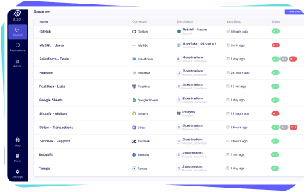
More and more I have been using Airbyte, an ELT tool (extract load transform) that loads all data as standard JSON, but also has an option of formatting your data, which in turn generates a dbt (data build tool) project where you can automate these transformations.

There are three steps here, but the first, of course, starts with turning your data into a CSV.

Install Airbyte

You can install Airbyte locally or in a cloud environment. You will need Docker installed but it is a simple three-step command to do so locally. You can find the guides in their docs:

Create a geospatial file source

The next step is to create a new source, specifically a File source to load your geospatial data.

Create a destination

Next, create a destination and enter the required credentials.

Establish your connection

Then, create your connection by connecting the source and destination, and make sure to select the option to normalize your data.

Extract, modify, and connect your dbt project

Once the sync has run you can generate and run the dbt project and files within Airbyte. This guide will show you how build and export the dbt project.

From here you can follow these steps once you have opened your project:

Run the dbt debug statement

dbt debug --profiles-dir /your_path/normalize

Install dbt dependencies

Modify the dbt_project.yml file to set a new dependencies location at packages-install-path:

Then run:

dbt deps --profiles-dir /your_path/normalize 

Modify the SQL file to create a geometry

Let’s start with a simple transformation to create a geometry in our table. Open the SQL file located at ../models/airbyte_tables/public/your_table_name.sql. You should see the dbt generated SQL here.

In this example, we are going to modify one line to create a geometry from the latitude and longitude columns. We need to cast the values to numeric within the ST_MakePoint function.

st_makepoint(cast(longitude as numeric), cast(latitude as numeric)) as geom

Of course, you can modify any part of this statement to adjust the data or add new columns. For repeatable data ingestion, this is extremely valuable as you can write this code once and then run the pipeline as needed. 

Run the new pipeline

Once you have saved your files, you can now run the new pipeline:

dbt run --profiles-dir /your_path/normalize 

Once this completes you should see your new column in your table in your data source.

Connect it to GitHub

Once you are happy with your results, you can load your dbt project to GitHub and connect this to your Airbyte connection, meaning that every time you run your sync, it will use this transformation going forward.